精品伊甸乐园入口xyz
福大主页
常用链接
联系我们
English
网站首页
学院概况
学院简介
党政领导
机构设置
办公机构
职能组织
师资队伍
院士风采
教师名录
教学团队
科研团队
行政思政
退休教师
学科建设
双一流建设学科
国家重点学科
211重点学科
优势学科平台
省重点学科
ESI期刊
人才培养
本科生教育
研究生教育
博士后流动站
国际化合作办学
科学研究
研究单位
通知公告
科研项目
获奖情况
论文成果
科研平台
党建工作
动态通知
党建公示
分党校
规章制度
理论学习
教工之家
工会概况
通知公告
工会动态
民主管理
学习园地
学校工会
退休家园
学生工作
新闻动态
通知公告
科技创新
就业创业
心理健康
风采展示
荣誉奖励
嘉锡班
校友园地
校庆活动
校友动态
校友风采
合作交流
校友墙
新闻中心
新闻动态
通知公告
学术活动
科研之窗
招生工作
博后招聘
人才招聘
院内信息
通知公告
重要文件
管理章程
岗位聘任
会议纪要
学院年报
文件下载
热门搜索:
本科生招生
研究生招生
27
2024-03
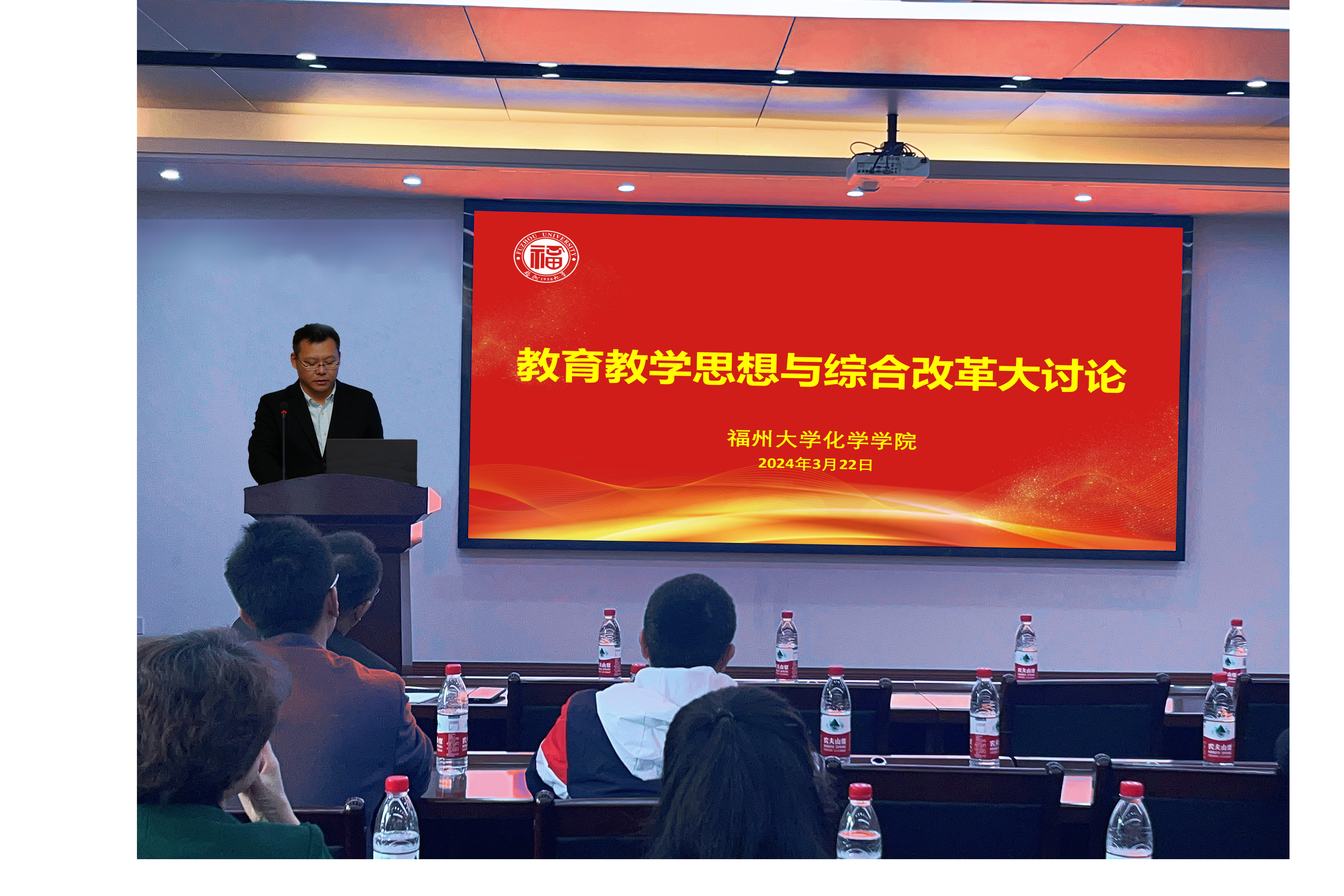
(3月22日)化学学院关于教育教学思想与综合改革大讨论系列讲座成功举行
25
2024-03
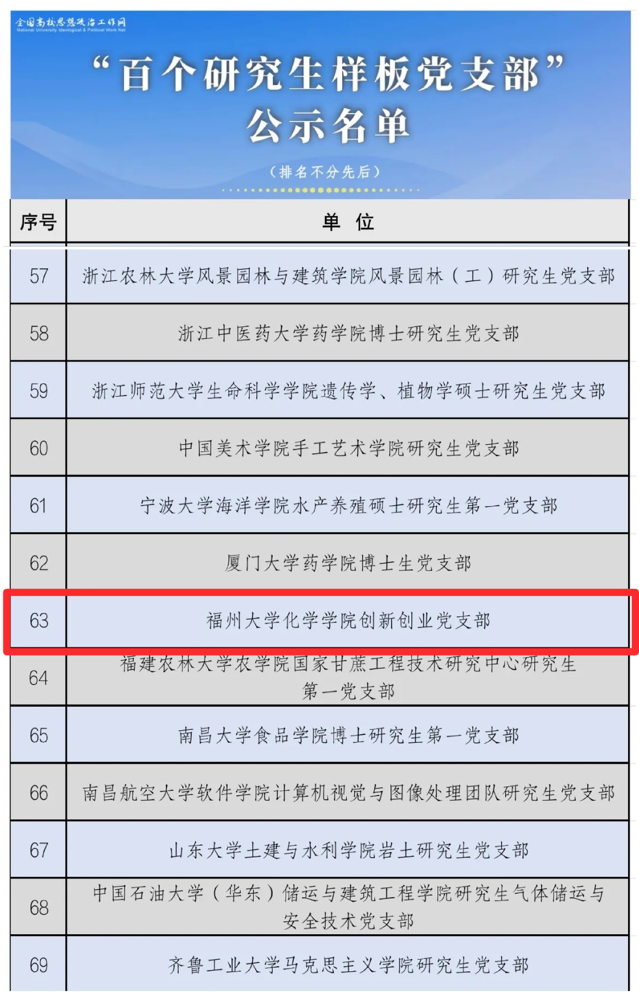
零的突破!化学学院在第三批全国高校研究生“双百”创建工作中取得双丰收!
25
2024-03
踏青寻春,“趣”享自然 | 化学学院开展2024年教职工春游活动
14
2024-03
“研究生教育管理”辅导员工作室组织参观卢嘉锡教育馆
04
2024-01
校长吴明红院士调研化学学院
16
2023-11
第二届理论与计算催化青年学者学术交流研讨会取得圆满成功
新闻动态
科研之窗
学院通知
2024-04-02
化学学院成功举办青年教师“最佳一节课”竞赛
2024-04-02
2024年化学学院最佳一节课获奖名单公示
2024-03-27
(3月22日)化学学院关于教育教学思想与综合改革大讨论系列讲座成功举行
2024-03-25
零的突破!化学学院在第三批全国高校研究生“双百”创建工作中取得双丰收!
2024-03-25
踏青寻春,“趣”享自然 | 化学学院开展2024年教职工春游活动
2024-03-19
研究生教育管理工作室组织开展辅导员科研能力提升培训活动
查看更多+
2024-01-11
我院宋秋玲教授课题组原创性成果在Nature Chemistry上发表
2023-12-23
我院林忠辉教授在《Nucleic Acids Res》和《EMBO J》连续发文揭示细菌III型CRISPR免疫系统的分子机制
2023-12-13
我院林振宇教授课题组近期研究工作概览
2023-12-12
我院黄兴教授课题组在ACS Nano上发表原位透射电子显微学研究及其对析氢反应的影响
2023-10-30
我院宋秋玲教授课题组近期在Chem、Nat Commun、Angew Chem、ACS Cat上发表5篇论文
2023-10-16
林森教授课题组在Angew Chem和JACS Au上发表关于催化物种动态演化的理论研究成果
查看更多+
2024-04-18
2024年精品伊甸乐园入口xyz硕士研究生复试拟录取结果公示(第三批次)
2024-04-16
福州大学关于开展2023-2024学年本科教学优秀奖评选工作的通知
2024-04-16
福州大学关于开展教学名师奖评选工作的通知
2024-04-15
精品伊甸乐园入口xyz2024年硕士研究生招生复试调剂公告(第三轮)
2024-04-13
精品伊甸乐园入口xyz2024年硕士研究生招生复试调剂公告(第二轮)
2024-04-13
2024年精品伊甸乐园入口xyz硕士研究生复试拟录取结果公示(第二批次)
查看更多+
数说化学
在读学生
2631
人
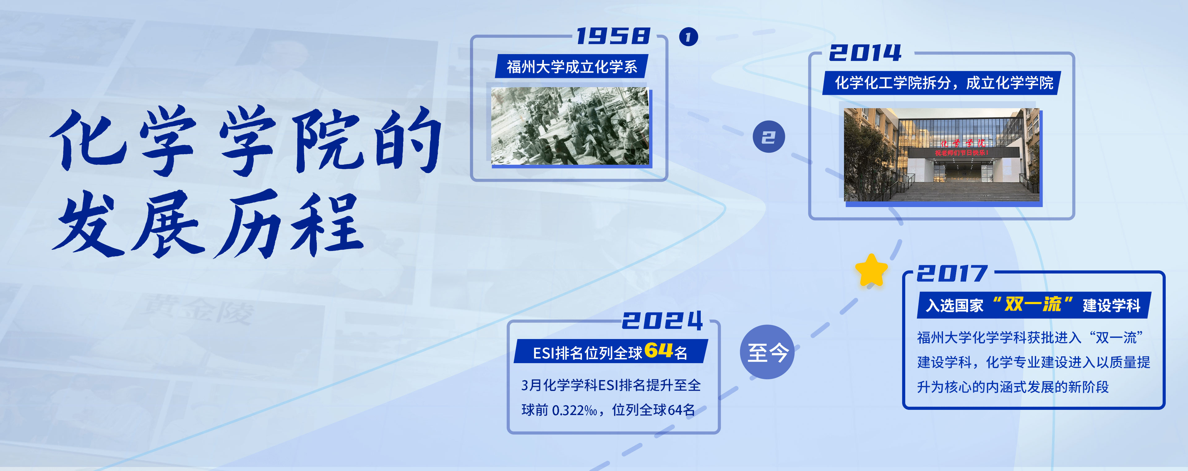
创院时间
1958
年
研究单位
15
个
专职教师
150
名
科技奖项
20
余项
科研平台
查看更多+
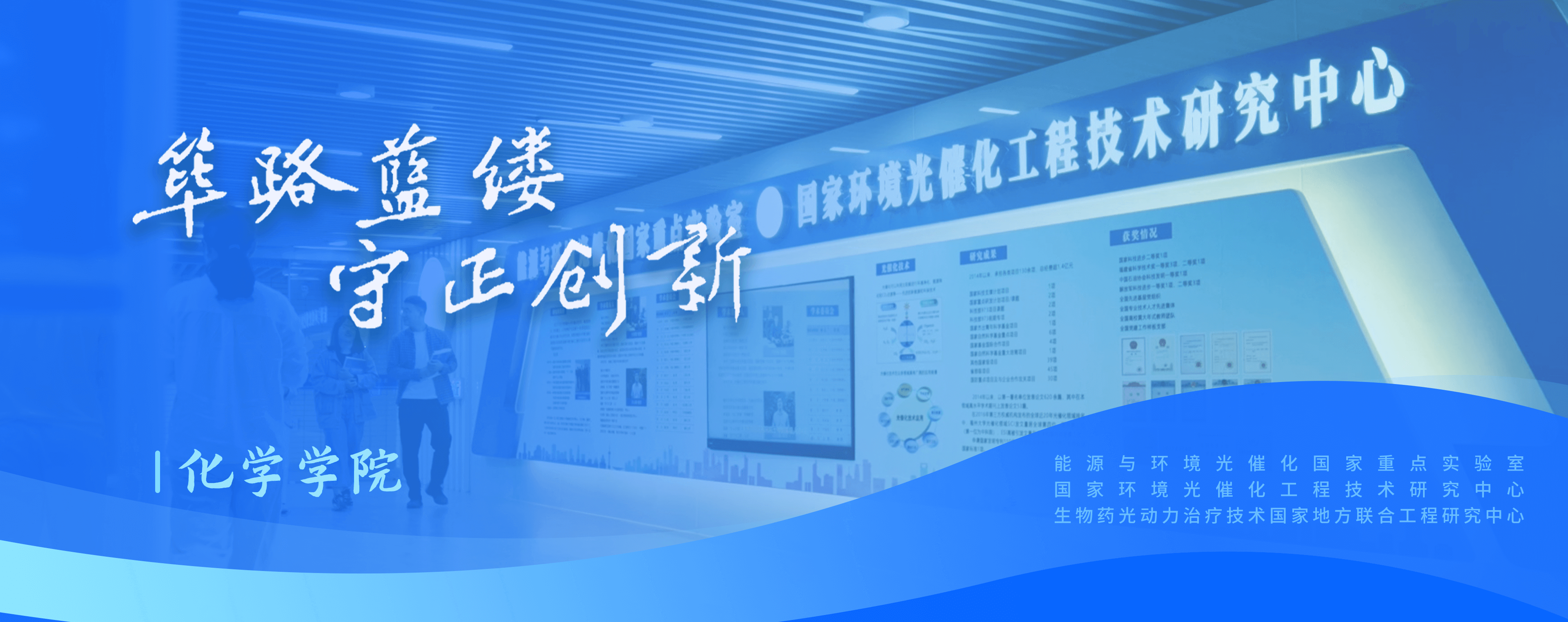
国家级科研平台
能源与环境光催化国家重点实验室
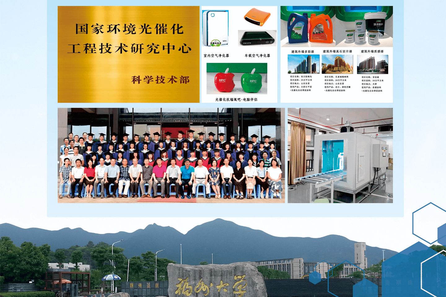
国家级科研平台
国家环境光催化工程技术研究中心
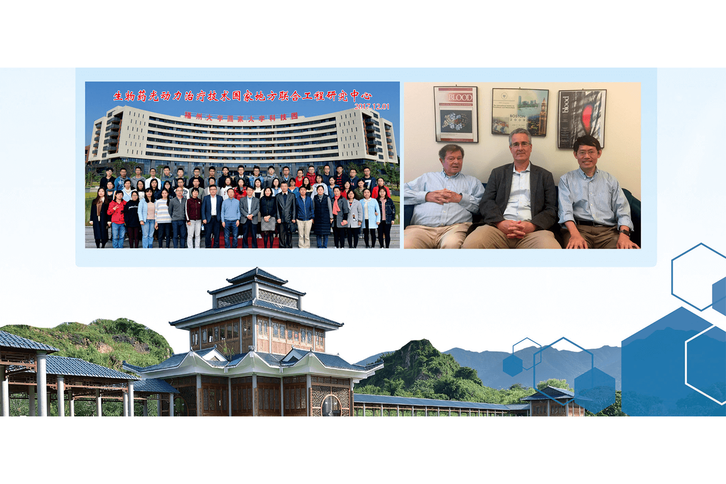
国家级科研平台
生物药光动力治疗技术国家地方联合
工程研究中心
学术讲座
查看更多+
19
2024-04
周五
(4月19日)响应型框架的多基元构筑和功能集成
上午09:30~上午11:30
章跃标,上海科技大学
嘉锡楼413
15
2024-04
周一
(4月15日)多酸团簇自组装及其性能研究
上午09:00~上午11:30
李中
嘉锡楼413
17
2024-04
周三
(4月17日)二维异质结结构电催化剂设计
上午10:00~上午11:30
陈佳义博士(新加坡国立大学生物分子与化学工程系)
科技园1号楼中401会议室
专题专栏
学术会议
会议室预约
研究生选课
本科生选课
实验教学中心
国际化办学
测试中心
下载专区


 新闻动态
新闻动态
 学院通知
学院通知


 上午09:30~上午11:30
 章跃标,上海科技大学
 嘉锡楼413